Odd Man Out: The Problem with Serpentine Drafts

In this article, we’re going to continue the trend of discussing topics related to Fantasy Sports. Specifically, the innate problem which I see within the serpentine draft format. I feel that this topic is particularly appropriate for this time of year, as football fans are gearing up for their own fantasy league drafts.

If you’re unfamiliar with the serpentine draft format, it is best described as:

A serpentine draft, or sometimes referred to as a a "Snake" draft, is a type in which the draft order is reversed every round (eg 1..12, 12..1, 1..12, 12..1, etc.). For example, if you have the first pick in the draft, you will pick first in round one, and then last in round two.

Source: https://help.fandraft.com/support/solutions/articles/61000278703-draft-types-and-formats

I’ve created a few examples of this draft type below. The innate issue which I see within this draft format, pertains to the differentiation between the projected point value of each draft selection, as determined by a team’s draft position. The more teams present within a league, the greater the point disparity between teams.

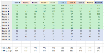
Assuming that each team executed an optimized drafting strategy, we would expect the outcome to resemble something like the illustration below.

Each number within a cell represents the best player value available to each team, each round. The green cells contain starting player values, and the grey cells contain back-up player values.

As you can observe from the summed values below each outcome column, each team possess a one point advantage against the team which selected subsequently, and a one point disadvantage against the team which selected previously. The greatest differentiation occurring between the team which made the first selection within the draft order, as measured against the team which made the last selection within the draft order: 11 (1026 – 1015).

As previously mentioned, the less teams within a league, the less the number of selection rounds. As a result of such, there is less of a disparity between the teams which pick earlier within the order, as compared to teams which pick later within the order.

Below is the optimal outcome of a league comprised of ten teams.

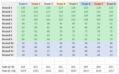
While the single point differentiation persists between consecutive teams within the draft order, the differentiation between the first selector, and the last selector, has been reduced to: 9 (856 – 847).

This trend continues across ever smaller league sizes: 7 (1024 – 1017).

In each instance, we should expect the total differentiation of points between the first draft participant, and last draft participant, (if optimal drafting occurred), to be equal to: N – 1. Where N = the number of total draft participants within the league.

All things being equal, if each team is managed optimally, we should expect the first team within each draft to finish first within each league. Second place would belong to the team which drafted second. Third place belonging to the team which drafted third, and so on, etc.

If all players are equally at risk of being injured on each fantasy team, then this occurrence does little to upset the overall ranking of teams by draft order. It must be remembered that teams which drafted earlier within the order, will also possess better replacement players as compared to their competitors. Therefore, when injuries do occur, later drafting teams will be disproportionately impacted.

I would imagine that as AI integration begins to seep into all aspects of existence, that the opportunity for each team owner to draft with consistent optimization, will further stratify the inherent edge attributed to serpentine draft position. As it stands currently, there is still an opportunity for lower draft order teams to compete if one or more of their higher order competitors blunder a selection. 

In any case, I hope that what I have written in this article helped to describe what I like to refer to as the, “Odd Man Out” phenomenon. I hope to see you again soon, with more of the statistical content which you crave.

-RD

(R) Daily Fantasy Sports Line-up Optimizer (Basketball)

I’ve been mulling over whether or not I should give away this secret sauce on my site, and I’ve come to the conclusion that anyone who seriously contends within the Daily Fantasy medium, probably is already aware of this strategy. 

Today, through the magic of R software, I will demonstrate how to utilize code to optimize your daily fantasy sports line-up. This particular example will be specific to the Yahoo daily fantasy sports platform, and to the sport of basketball.

I also want to give credit, where credit is due.

The code presented below is a heavily modified variation of code initially created by: Patrick Clark.

The original code source case be found here: http://patrickclark.info/Lineup_Optimizer.html

Example:

First, you’ll need to access Yahoo’s Daily Fantasy page. I’ve created an NBA Free QuickMatch, which is a 1 vs. 1 contest against an opponent where no money changes hands.

This page will look a bit different during the regular season, as the NBA playoffs are currently underway. That aside, our next step is to download all of the current player data. This can be achieved by clicking on the “i” bubble icon.



Next, click on the “Export players list” link. This will download the previously mentioned player data.

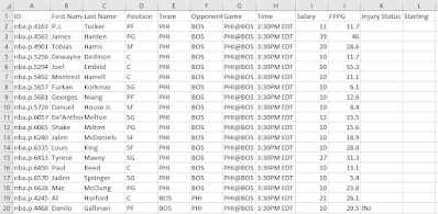
The player data should resemble the (.csv) image below:



Prior to proceeding to the subsequent step, we need to do a bit of manual data clean up.

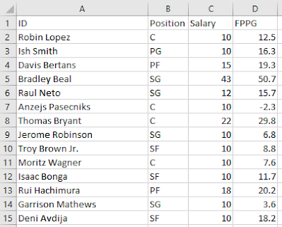
Any player who is injured or not starting, I removed from the data set. I also concatenated the First Name and Last Name fields, and placed that concatenation within the ID variable. Next, I removed all variables except for the following: ID (newly modified), Position, Salary, and FPPG (Fantasy Points Per Game).

The results should resemble the following image:



(Specific player data and all associated variables will differ depending on the date of download)

Now that the data has been formatted, we’re ready to code!

###################################################################

library(lpSolveAPI)

library(tidyverse)

# It is easier to input the data as an Excel file if possible #

# Player names (ID) have the potential to upset the .CSV format #

library(readxl)

# Be sure to set the played data file path to match your directory / file name #

PlayerPool <- read_excel("C:/Users/Your_Modified_Players_List.xlsx")

# Create some positional identifiers in the pool of players to simplify linear constraints #

# This code creates new position column variables, and places a 1 if a player qualifies for a position #

PlayerPool$PG_Check <- ifelse(PlayerPool$Position == "PG",1,0)

PlayerPool$SG_Check <- ifelse(PlayerPool$Position == "SG",1,0)

PlayerPool$SF_Check <- ifelse(PlayerPool$Position == "SF",1,0)

PlayerPool$PF_Check <- ifelse(PlayerPool$Position == "PF",1,0)

PlayerPool$C_Check <- ifelse(PlayerPool$Position == "C",1,0)

PlayerPool$One <- 1

# This code modifies the position columns so that each variable is a vector type #

PlayerPool$PG_Check <- as.vector(PlayerPool$PG_Check)

PlayerPool$SG_Check <- as.vector(PlayerPool$SG_Check)

PlayerPool$SF_Check <- as.vector(PlayerPool$SF_Check)

PlayerPool$PF_Check <- as.vector(PlayerPool$PF_Check)

PlayerPool$C_Check <- as.vector(PlayerPool$C_Check)

# This code orders each player ID by position #

PlayerPool <- PlayerPool[order(PlayerPool$PG_Check),]

PlayerPool <- PlayerPool[order(PlayerPool$SG_Check),]

PlayerPool <- PlayerPool[order(PlayerPool$SF_Check),]

PlayerPool <- PlayerPool[order(PlayerPool$PF_Check),]

PlayerPool <- PlayerPool[order(PlayerPool$C_Check),]

# Appropriately establish variables in order to perform the "solver" function #

Num_Players <- length(PlayerPool$One)

lp_model = make.lp(0, Num_Players)

set.objfn(lp_model, PlayerPool$FPPG)

lp.control(lp_model, sense= "max")

set.type(lp_model, 1:Num_Players, "binary")

# Total salary points avalible to the player #

# In the case of Yahoo, the salary points are set to ($)200 #

add.constraint(lp_model, PlayerPool$Salary, "<=",200)

# Maximum / Minimum Number of Players necessary for each position type #

add.constraint(lp_model, PlayerPool$PG_Check, "<=",3)

add.constraint(lp_model, PlayerPool$PG_Check, ">=",1)

# Maximum / Minimum Number of Players necessary for each position type #

add.constraint(lp_model, PlayerPool$SG_Check, "<=",3)

add.constraint(lp_model, PlayerPool$SG_Check, ">=",1)

# Maximum / Minimum Number of Players necessary for each position type #

add.constraint(lp_model, PlayerPool$SF_Check, "<=",3)

add.constraint(lp_model, PlayerPool$SF_Check, ">=",1)

# Maximum / Minimum Number of Players necessary for each position type #

add.constraint(lp_model, PlayerPool$PF_Check, "<=",3)

add.constraint(lp_model, PlayerPool$PF_Check, ">=",1)

# Maximum / Minimum Number of Players necessary for each position type (only require one (C)enter) #

add.constraint(lp_model, PlayerPool$C_Check, "=",1)

# Total Numner of Players Needed for the entire Fantasy Line-up #

add.constraint(lp_model, PlayerPool$One, "=",8)

# Perform the Solver function #

solve(lp_model)

# Projected_Score provides the projected score summed from the optimized projected line-up (FPPG) #

Projected_Score <- crossprod(PlayerPool$FPPG,get.variables(lp_model))

get.variables(lp_model)

# The optimal_lineup data frame provides the optimized line-up selection #

optimal_lineup <- subset(data.frame(PlayerPool$ID, PlayerPool$Position, PlayerPool$Salary), get.variables(lp_model) == 1)

If we take a look at our:

Projected_Score

We should receive an output which resembles the following:

> Projected_Score
    [,1]
[1,] 279.5

Now, let’s take a look at our:

optimal_lineup

Our output should resemble something like:

PlayerPool.ID PlayerPool.Position PlayerPool.Salary
3 Marcus Smart PG 20
51 Bradley Beal SG 43
108 Tyrese Haliburton SG 16
120 Jerami Grant SF 27
130 Eric Gordon SF 19
148 Brandon Ingram SF 36
200 Darius Bazley PF 19
248 Steven Adams C 20

With the above information, we are prepared to set our line up.

You could also run this line of code:

optimal_lineup <- subset(data.frame(PlayerPool$ID, PlayerPool$Position, PlayerPool$Salary, PlayerPool$FPPG), get.variables(lp_model) == 1)

optimal_lineup

Which provides a similar output that also includes point projections:

PlayerPool.ID PlayerPool.Position PlayerPool.Salary PlayerPool.FPPG
3 Marcus Smart PG 20 29.8
51 Bradley Beal SG 43 50.7
108 Tyrese Haliburton SG 16 26.9
120 Jerami Grant SF 27 38.4
130 Eric Gordon SF 19 30.7
148 Brandon Ingram SF 36 43.2
200 Darius Bazley PF 19 29.7
248 Steven Adams C 20 30.1

Summing up PlayerPool.FPPG, we reach the value: 279.5. This was the same value which we observed within the Projected_Score matrix.

Conclusion:

While this article demonstrates a very interesting concept, I would be remiss if I did not advise you to NOT gamble on daily fantasy. This post was all in good fun, and for educational purposes only. By all means, defeat your friends and colleagues in free leagues, but do not turn your hard-earned money over to gambling websites.

The code presented within this entry may provide you with a minimal edge, but shark players are able to make projections based on far more robust data sets as compared to league FPPG. 

In any case, the code above can be repurposed for any other daily fantasy sport (football, soccer, hockey, etc.). Remember, only to play for fun and for free. 

-RD 

(R) Bedford's Law

In today’s article, we will be discussing Benford’s Law, specifically as it is utilized as an applied methodology to assess financial documents for potential fraud:

First, a bit about the phenomenon which Benford sought to describe:

The discovery of Benford's law goes back to 1881, when the Canadian-American astronomer Simon Newcomb noticed that in logarithm tables the earlier pages (that started with 1) were much more worn than the other pages. Newcomb's published result is the first known instance of this observation and includes a distribution on the second digit, as well. Newcomb proposed a law that the probability of a single number N being the first digit of a number was equal to log(N + 1) − log(N).

The phenomenon was again noted in 1938 by the physicist Frank Benford, who tested it on data from 20 different domains and was credited for it. His data set included the surface areas of 335 rivers, the sizes of 3259 US populations, 104 physical constants, 1800 molecular weights, 5000 entries from a mathematical handbook, 308 numbers contained in an issue of Reader's Digest, the street addresses of the first 342 persons listed in American Men of Science and 418 death rates. The total number of observations used in the paper was 20,229. This discovery was later named after Benford (making it an example of Stigler's law).

Source: https://en.wikipedia.org/wiki/Benford%27s_law

So what does this actually mean in laymen’s terms?

Essentially, given a series of numerical elements from a similar source, we should expect certain leading digits to occur, and correspond to, a particular distribution patter. 



If a series of elements perfectly corresponds with Benford’s Law, then the elements within the series should follow the above pattern as it pertains to leading digit frequency. Ex. Numbers which begin the number “1”, should occur 30.1% of the time. Numbers which begin with the number “2”, should occur 17.6% of the time. Numbers which begin with the number “3”, should occur 12.5% of the time.

The distribution is derived as follows:



The utilization of Benford’s Law is applicable to numerous scenarios:

1. Accounting fraud detection

2. Use in criminal trials

3. Election data 

4. Macroeconomic data

5. Election data 

6. Price digit analysis 

7. Genome data 

8. Scientific fraud detection 

As it relates to screening for financial fraud, if the application of methodology related to the Benford’s Law Distribution returns a result in which the sample elements do not correspond with the distribution, then fraud is not necessarily the conclusion which we would immediately assume. However, the findings may indicate that additional data scrutinization is necessary. 

Example:

Let’s utilize Benford’s Law to analyze Cloudflare’s (NET) Balance Sheet (12/31/2021).



Even though it’s an un-necessary step as it relates to our analysis, let’s first discern the frequency of each leading digit. These digits are underlined in red within the graphic above.



What Benford’s Law will seeks to assess, is the comparison of leading digits as they occurred within our experiment, to our expectations as they exist within the Benford’s Law Distribution.



The above table illustrates the frequency of occurrence of each leading digit within our analysis, versus the expected percentage frequency as stated by Benford’s Law.

Now let’s perform the analysis:

# H0: The first digits within the population counts follow Benford's law #

# H1: The first digits within the population counts do not follow Benford's law #

# requires benford.analysis #

library(benford.analysis)

# Element entries were gathered from Cloudflare’s (NET) Balance Sheet (12/31/2021) #

NET <- c(2372071.00, 1556273.00, 815798.00, 1962675.00, 815798.00, 134212.00, 791014.00, 1667291.00, 1974792.00, 791014.00, 1293206.00, 845217.00, 323612.00, 323612.00)

# Perform Analysis #

trends <- benford(NET, number.of.digits = 1, sign = "positive", discrete=TRUE, round=1)

# Display Analytical Output #

trends

# Plot Analytical Findings #

plot(trends)

Which provides the output:

Benford object:

Data: NET
Number of observations used = 14
Number of obs. for second order = 10
First digits analysed = 1

Mantissa:

Statistic Value
    Mean 0.51
    Var 0.11
Ex.Kurtosis -1.61
    Skewness 0.25

The 5 largest deviations:

digits absolute.diff
1 8 2.28
2 1 1.79
3 2 1.47
4 4 1.36
5 7 1.19

Stats:

Pearson's Chi-squared test

data: NET
X-squared = 14.729, df = 8, p-value = 0.06464

Mantissa Arc Test

data: NET
L2 = 0.092944, df = 2, p-value = 0.2722

Mean Absolute Deviation (MAD): 0.08743516
MAD Conformity - Nigrini (2012): Nonconformity
Distortion Factor: 8.241894

Remember: Real data will never conform perfectly to Benford's Law. You should not focus on p-values!

~ Graphical Output Provided by Function ~

(The most important aspects of the output are bolded)

Findings:

Pearson's Chi-squared test

data: NET
X-squared = 14.729, df = 8, p-value = 0.06464
Remember: Real data will never conform perfectly to Benford's Law. You should not focus on p-values!



A chi-square goodness of fit test was performed to examine whether the first digit of balance sheet items from the company Cloudflare (12/31/2021), adhere to Benford's law. Entries were found to be in adherence, with non-significance at the p < .05 level, χ2 (8, N = 14) = 14.73, p = 0.07.

As it relates to the graphic, in ideal circumstances, each blue data bar should have its uppermost portion touching the broken red line.

Example(2):

If you’d prefer to instead run the analysis simply as a chi-squared test which does not require the “benford.analysis” package, you can effectively utilize the following code. The image below demonstrates the concept being employed.



Model <- c(6, 1, 2, 0, 0, 0, 2, 3, 0)

Results <- c(0.30102999566398100, 0.17609125905568100, 0.12493873660830000, 0.09691001300805650, 0.07918124604762480, 0.06694678963061320, 0.05799194697768670, 0.05115252244738130, 0.04575749056067510)

chisq.test(Model, p=Results, rescale.p = FALSE)

Which provides the output:

    Chi-squared test for given probabilities

data: Model
X-squared = 14.729, df = 8, p-value = 0.06464

Which are the same findings that we encountered while performing the analysis previously.

That’s all for now! Stay studious, Data Heads! 

-RD